Gaussian Process Regression

Zhenwen Dai (2019-05-29)

Introduction

Gaussian process (GP) is a Bayesian non-parametric model used for various machine learning problems such as regression, classification. This notebook shows about how to use a Gaussian process regression model in MXFusion.

import warnings
warnings.filterwarnings('ignore')
import os
os.environ['MXNET_ENGINE_TYPE'] = 'NaiveEngine'

Toy data

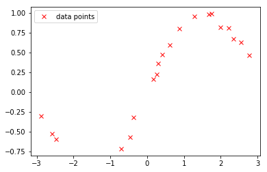
We generate some synthetic data for our regression example. The data set is generate from a sine function with some additive Gaussian noise.

import numpy as np
%matplotlib inline
from pylab import *

np.random.seed(0)
X = np.random.uniform(-3.,3.,(20,1))
Y = np.sin(X) + np.random.randn(20,1)*0.05

The generated data are visualized as follows:

plot(X, Y, 'rx', label='data points')
_=legend()

Gaussian process regression with Gaussian likelihood

Denote a set of input points \(X \in \mathbb{R}^{N \times Q}\). A Gaussian process is often formulated as a multi-variate normal distribution conditioned on the inputs:

\[ \begin{align}\begin{aligned} p(F|X) = \mathcal{N}(F; 0, K),\\where :math:`F \in \mathbb{R}^{N \times 1}` is the corresponding output points of the Gaussian process and :math:`K` is the covariance matrix computed on the set of inputs according to a chosen kernel function :math:`k(\cdot, \cdot)`.\end{aligned}\end{align} \]

For a regression problem, \(F\) is often referred to as the noise-free output and we usually assume an additional probability distribution as the observation noise. In this case, we assume the noise distribution to be Gaussian:

\[ \begin{align}\begin{aligned} p(Y|F) = \mathcal{N}(Y; F, \sigma^2 \mathcal{I}),\\where :math:`Y \in \mathbb{R}^{N \times 1}` is the observed output and :math:`\sigma^2` is the variance of the Gaussian distribution.\end{aligned}\end{align} \]

The following code defines the above GP regression in MXFusion. First, we change the default data dtype to double precision to avoid any potential numerical issues.

from mxfusion.common import config
config.DEFAULT_DTYPE = 'float64'

In the code below, the variable Y is defined following the probabilistic module GPRegression. A probabilistic module in MXFusion is a pre-built probabilistic model with dedicated inference algorithms for computing log-pdf and drawing samples. In this case, GPRegression defines the above GP regression model with a Gaussian likelihood. It understands that the log-likelihood after marginalizing \(F\) is closed-form and exploits this property when computing log-pdf.

The model is defined by the input variable X with the shape (m.N, 1), where the value of m.N is discovered when data is given during inference. A positive noise variance variable m.noise_var is defined with the initial value to be 0.01. For GP, we define a RBF kernel with input dimensionality being one and initial value of variance and lengthscale to be one. We define the variable m.Y following the GP regression distribution with the above specified kernel, input variable and noise_variance.

from mxfusion import Model, Variable
from mxfusion.components.variables import PositiveTransformation
from mxfusion.components.distributions.gp.kernels import RBF
from mxfusion.modules.gp_modules import GPRegression

m = Model()
m.N = Variable()
m.X = Variable(shape=(m.N, 1))
m.noise_var = Variable(shape=(1,), transformation=PositiveTransformation(), initial_value=0.01)
m.kernel = RBF(input_dim=1, variance=1, lengthscale=1)
m.Y = GPRegression.define_variable(X=m.X, kernel=m.kernel, noise_var=m.noise_var, shape=(m.N, 1))

In the above model, we have not defined any prior distributions for any hyper-parameters. To use the model for regrssion, we typically do a maximum likelihood estimate for all the hyper-parameters conditioned on the input and output variable. In MXFusion, this is done by first creating an inference algorithm, which is MAP in this case, by specifying the observed variables. Then, we create an inference body for gradient optimization inference methods, which is called GradBasedInference. The inference method is triggered by calling the run method, in which all the observed data are given as keyword arguments and any necessary configruation parameters are specified.

import mxnet as mx
from mxfusion.inference import GradBasedInference, MAP

infr = GradBasedInference(inference_algorithm=MAP(model=m, observed=[m.X, m.Y]))
infr.run(X=mx.nd.array(X, dtype='float64'), Y=mx.nd.array(Y, dtype='float64'),
         max_iter=100, learning_rate=0.05, verbose=True)

Iteration 10 loss: -13.09287954321266
Iteration 20 loss: -15.971970034359586
Iteration 30 loss: -16.725359053995163
Iteration 40 loss: -16.835084442759314
Iteration 50 loss: -16.850332113428053
Iteration 60 loss: -16.893812683762203
Iteration 70 loss: -16.900137667771077
Iteration 80 loss: -16.901158761459012
Iteration 90 loss: -16.903085976668137
Iteration 100 loss: -16.903135093930537

All the inference outcomes are in the attribute params of the inference body. The inferred value of a parameter can be access by passing the reference of the queried parameter to the params attribute. For example, to get the value m.noise_var, we can call inference.params[m.noise_var]. The estimated parameters from the above experiment are as follows:

print('The estimated variance of the RBF kernel is %f.' % infr.params[m.kernel.variance].asscalar())
print('The estimated length scale of the RBF kernel is %f.' % infr.params[m.kernel.lengthscale].asscalar())
print('The estimated variance of the Gaussian likelihood is %f.' % infr.params[m.noise_var].asscalar())

The estimated variance of the RBF kernel is 0.616992.
The estimated length scale of the RBF kernel is 1.649073.
The estimated variance of the Gaussian likelihood is 0.002251.

We can compare the estimated values with the same model implemented in GPy. The estimated values from GPy are very close to the ones from MXFusion.

import GPy

m_gpy = GPy.models.GPRegression(X, Y, kernel=GPy.kern.RBF(1))
m_gpy.optimize()
print(m_gpy)

Name : GP regression
Objective : -16.903456670910902
Number of Parameters : 3
Number of Optimization Parameters : 3
Updates : True
Parameters:
  GP_regression.           |                 value  |  constraints  |  priors
  rbf.variance             |    0.6148038604494702  |      +ve      |
  rbf.lengthscale          |    1.6500299722611123  |      +ve      |
  Gaussian_noise.variance  |  0.002270049772204339  |      +ve      |

Prediction

The above section shows how to estimate the model hyper-parameters of a GP regression model. This is often referred to as training. After training, we are often interested in using the inferred model to predict on unseen inputs. The GP modules offers two types of predictions: predicting the mean and variance of the output variable or drawing samples from the predictive posterior distributions.

Mean and variance of the posterior distribution

To estimate the mean and variance of the predictive posterior distribution, we use the inference algorithm ModulePredictionAlgorithm, which takes the model, the observed variables and the target variables of prediction as input arguments. We use TransferInference as the inference body, which allows us to take the inference outcome from the previous inference. This is done by passing the inference parameters infr.params into the infr_params argument.

from mxfusion.inference import TransferInference, ModulePredictionAlgorithm
infr_pred = TransferInference(ModulePredictionAlgorithm(model=m, observed=[m.X], target_variables=[m.Y]),
                              infr_params=infr.params)

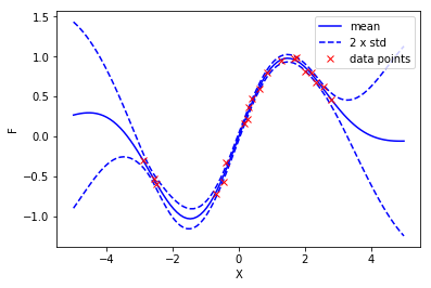
To visualize the fitted model, we make predictions on 100 points evenly spanned from -5 to 5. We estimate the mean and variance of the noise-free output \(F\).

xt = np.linspace(-5,5,100)[:, None]
res = infr_pred.run(X=mx.nd.array(xt, dtype='float64'))[0]
f_mean, f_var = res[0].asnumpy()[0], res[1].asnumpy()[0]

The resulting figure is shown as follows:

plot(xt, f_mean[:,0], 'b-', label='mean')
plot(xt, f_mean[:,0]-2*np.sqrt(f_var), 'b--', label='2 x std')
plot(xt, f_mean[:,0]+2*np.sqrt(f_var), 'b--')
plot(X, Y, 'rx', label='data points')
ylabel('F')
xlabel('X')
_=legend()

Posterior samples of Gaussian process

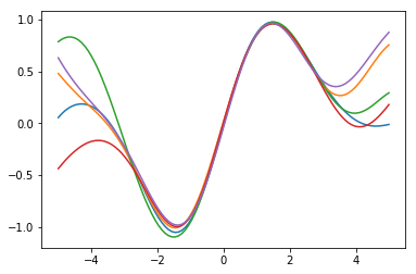
Apart from getting the mean and variance at every location, we may need to draw samples from the posterior GP. As the output variables at different locations are correlated with each other, each sample gives us some idea of a potential function from the posterior GP distribution.

To draw samples from the posterior distribution, we need to change the prediction inference algorithm attached to the GP module. The default prediction function estimate the mean and variance of the output variable as shown above. We can attach another inference algorithm as the prediction algorithm. In the following code, we attach the GPRegressionSamplingPrediction algorithm as the prediction algorithm. The targets and conditionals arguments specify the target variables of the algorithm and the conditional variables of the algorithm. After spcifying a name in the alg_name argument such as gp_predict, we can access this inference algorithm with the specified name like gp.gp_predict. In following code, we set the diagonal_variance attribute to be False in order to draw samples from a full covariace matrix. To avoid numerical issue, we set a small jitter to help matrix inversion. Then, we create the inference body in the same way as the above example.

from mxfusion.inference import TransferInference, ModulePredictionAlgorithm
from mxfusion.modules.gp_modules.gp_regression import GPRegressionSamplingPrediction

gp = m.Y.factor
gp.attach_prediction_algorithms(targets=gp.output_names, conditionals=gp.input_names,
            algorithm=GPRegressionSamplingPrediction(
                gp._module_graph, gp._extra_graphs[0], [gp._module_graph.X]),
            alg_name='gp_predict')
gp.gp_predict.diagonal_variance = False
gp.gp_predict.jitter = 1e-8
infr_pred = TransferInference(ModulePredictionAlgorithm(model=m, observed=[m.X], target_variables=[m.Y], num_samples=5),
                              infr_params=infr.params)

We draw five samples on the 100 evenly spanned input locations.

xt = np.linspace(-5,5,100)[:, None]
y_samples = infr_pred.run(X=mx.nd.array(xt, dtype='float64'))[0].asnumpy()

We visualize the individual samples each with a different color.

for i in range(y_samples.shape[0]):
    plot(xt, y_samples[i,:,0])

Gaussian process with a mean function

In the previous example, we created an GP regression model without a mean function (the mean of GP is zero). It is very easy to extend a GP model with a mean field. First, we create a mean function in MXNet (a neural network). For simplicity, we create a 1D linear function as the mean function.

mean_func = mx.gluon.nn.Dense(1, in_units=1, flatten=False)
mean_func.initialize(mx.init.Xavier(magnitude=3))

We create the GP regression model in a similar way as above. The difference is 1. We create a wrapper of the mean function in model definition m.mean_func. 2. We evaluate the mean function with the input of our GP model, which results into the mean of the GP. 3. We pass the resulting mean into the mean argument of the GP module.

m = Model()
m.N = Variable()
m.X = Variable(shape=(m.N, 1))
m.mean_func = MXFusionGluonFunction(mean_func, num_outputs=1, broadcastable=True)
m.mean = m.mean_func(m.X)
m.noise_var = Variable(shape=(1,), transformation=PositiveTransformation(), initial_value=0.01)
m.kernel = RBF(input_dim=1, variance=1, lengthscale=1)
m.Y = GPRegression.define_variable(X=m.X, kernel=m.kernel, noise_var=m.noise_var, mean=m.mean, shape=(m.N, 1))

import mxnet as mx
from mxfusion.inference import GradBasedInference, MAP

infr = GradBasedInference(inference_algorithm=MAP(model=m, observed=[m.X, m.Y]))
infr.run(X=mx.nd.array(X, dtype='float64'), Y=mx.nd.array(Y, dtype='float64'),
         max_iter=100, learning_rate=0.05, verbose=True)

Iteration 10 loss: -6.288699675985622
Iteration 20 loss: -13.938366520031717
Iteration 30 loss: -16.238146742572965
Iteration 40 loss: -16.214515784955303
Iteration 50 loss: -16.302410205174386
Iteration 60 loss: -16.423765889507315
Iteration 70 loss: -16.512277794947106
Iteration 80 loss: -16.5757306621185
Iteration 90 loss: -16.6410597628529
Iteration 100 loss: -16.702913078848557

from mxfusion.inference import TransferInference, ModulePredictionAlgorithm
infr_pred = TransferInference(ModulePredictionAlgorithm(model=m, observed=[m.X], target_variables=[m.Y]),
                              infr_params=infr.params)

xt = np.linspace(-5,5,100)[:, None]
res = infr_pred.run(X=mx.nd.array(xt, dtype='float64'))[0]
f_mean, f_var = res[0].asnumpy()[0], res[1].asnumpy()[0]

plot(xt, f_mean[:,0], 'b-', label='mean')
plot(xt, f_mean[:,0]-2*np.sqrt(f_var), 'b--', label='2 x std')
plot(xt, f_mean[:,0]+2*np.sqrt(f_var), 'b--')
plot(X, Y, 'rx', label='data points')
ylabel('F')
xlabel('X')
_=legend()

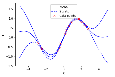
The effect of the mean function is not noticable, because there is no linear trend in our data. We can plot the values of the estimated parameters of the linear mean function.

print("The weight is %f and the bias is %f." %(infr.params[m.mean_func.parameters['dense1_weight']].asnumpy(),
                                               infr.params[m.mean_func.parameters['dense1_bias']].asscalar()))

The weight is 0.021969 and the bias is 0.079038.

Variational sparse Gaussian process regression

In MXFusion, we also have variational sparse GP implemented as a module. A sparse GP model can be created in a similar way as the plain GP model.

from mxfusion import Model, Variable
from mxfusion.components.variables import PositiveTransformation
from mxfusion.components.distributions.gp.kernels import RBF
from mxfusion.modules.gp_modules import SparseGPRegression

m = Model()
m.N = Variable()
m.X = Variable(shape=(m.N, 1))
m.noise_var = Variable(shape=(1,), transformation=PositiveTransformation(), initial_value=0.01)
m.kernel = RBF(input_dim=1, variance=1, lengthscale=1)
m.Y = SparseGPRegression.define_variable(X=m.X, kernel=m.kernel, noise_var=m.noise_var, shape=(m.N, 1), num_inducing=50)